Introduction
For the last week or so I’ve been moving to a new apartment, and thus haven’t had Internet access. I wanted to work on something in the evenings to pass the time, but the project had to be doable without looking up resources online. I decided to explore random number generation in video games, based on my cursory understanding of how it’s implemented in Dota.
Games often introduce random elements to make combat more interesting. For example, a certain character may have a 25% chance to do double damage when attacking an enemy — this is typically referred to a critical hit or a crit. Similar modifiers, such as slows or bashes, can also be applied randomly. In video game terminology a successfully applied modifier is referred to as a proc, which stands for Programmed Random OCcurance.
Uniform Distribution
Implementing attack modifiers using a uniform random number source is quite straightforward. Given a probability to proc c and a random number generator U, the game simply needs to evaluate the following for each attack:
If the expression is true the modifier is applied, otherwise it isn’t. For the rest of this post, I’ll refer to that technique as using a pseudo-random number generator (PRNG). Under the hood, software random number sources like rand() and drand48() use a deterministic algorithm that only appears random, hence the pseudo.
The problem with using a PRNG is that uniform randomness is actually too unpredictable. Especially in games like Dota and League of Legends, both of which are played professionally, it’s important for modifiers proc in a somewhat predictable way. The situations that need to be avoided are sequences of many repeated procs, and the opposite where a modifier isn’t applied for a long period of time. For example, consider a crit that’s applied to an attack with a probability of 30%. Given a large enough sample size, it’s not unreasonable to see sequences of 7 or 8 attacks without the effect occurring at all. Human intuition would expect a proc every 3 or 4 attacks, based on the 30% probability. Note the large gaps that occur in the sample graph below, and the region with many repeated events on the right side of the graph:
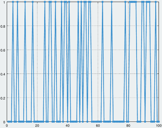
Simulation of a 30% probability modifier using a uniform distribution. A 1.0 on the y axis indicates a proc, and the x axis indicates the sample number
Uniform distributions are most effective when a large number of samples are taken — in the above graph, the frequency of procs is very close to 30/100. However, video game players are primarily concerned with shorter sequences of events not long term statistics. In combat a player may only be able to get off a handful of attacks before dying or being forced to retreat. As such, it’s important for the 30% probability to be relevant for smaller sequences, such as 5 to 10 attacks.
A more refined approach capable of accounting for past events is necessary. If a modifier doesn’t proc for several attacks, it should be more likely proc in the near future. Of course, whatever system is used can’t be too predictable either, else there would be no point in using random elements at all. It shouldn’t be possible to determine exactly when an effect will be applied.
Quasi Random Distribution
In the Dota documentation the technique of using a non-uniform distribution is typically referred to as a pseudo-random distribution. While the name is technically correct, I prefer the term quasi-random distribution for a variety of reasons. Firstly, it more easily differentiates the technique from the PRNGs used in most software applications. Secondly, and more importantly, it highlights that its main purpose is to generate low-discrepancy sequences.
The following sample data was generated using my quasi-random number generator (QRNG) approach. The effective probability of the distribution, which is explained in a later section, was close to 30%. In the macro scale this means the distribution behaves much like the uniform distribution shown earlier, however short subsequences have more consistent behavior.
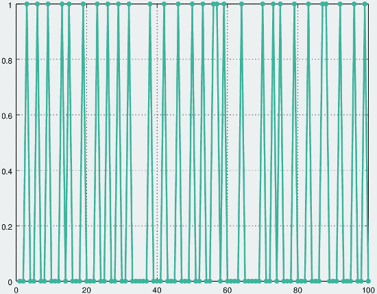
Simulation of a 30% probability modifier using a quasi-random distribution. A 1.0 on the y axis indicates a proc, and the a x axis indicates the sample number
It’s possible to get multiple procs in a row and to have runs with no modifier applied, however the large gaps seen the uniform distribution are very unlikely.
Initial Attempts
When I first set out to implement a QRNG my initial approach was to use some sort of card drawing technique. For example, for a modifier with a 25% chance a deck of eight cards could be used. The deck would contain two proc cards, and six regular, non-procing cards. The cards are shuffled and a card is drawn without replacement on each attack. A proc card results in the modifier being applied to attack, while a regular results in a normal unmodified attack. Once the deck is depleted, e.g. eight attacks have occurred, it is reshuffled and the process is repeated. Of course, cards are simply a metaphor to visualize the behavior of the algorithm.
The problem with this technique is that it’s possibly too predictable. If a player is aware of the underlying mechanism they can use it to make an informed prediction of future events, almost like counting cards. Additionally the approach doesn’t scale well for proc chances with fractional parts or prime numbers — probability of 17% requires a deck size of 100 cards. The same problems from the the uniform distribution start to crop in with decks of that size.
I don’t have any concrete data for the technique as I discarded the idea before writing any code. It seemed worth mentioning, however, since it may be appropriate under certain circumstances.
State Machine Approach
Background
The technique that I ended developing uses a state machine, where each state contains a different proc probability. When performing an attack the probability in the current state is used to determine if a modifier should be applied. If the modifier procs the state machine resets back to the initial state, and if the modifier fails to be applied it advances to the next state.
The overall idea is that as more attacks occur without a proc, the modifier has a increasing high chance of occurring on the next attack. The initial state is assigned a base probability value, and each subsequent state has a probability that is incrementally higher than the previous one. I also included a maximum state probability; when a state reaches the maximum value the forward edge simply loops back into that state.
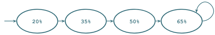
An example state machine, with a base probability of 20%, increment of 15% and max of 65%. Back edges are left off for simplicity
When implementing the QRNG in code, the state machine can be thought of as a sequence of numbers in an array or as a function that produces state probabilities based on the state index. It’s unnecessary to use a graph structure to evaluate the probabilities.
Formulation
The technique uses three parameters, a base probability b, an increment i and a max probability m. The sequence of probabilities in the state machine can be defined as follows, where R(x) is the value at state number x. The initial state is x=0.
The conditional probability of a proc occurring at a given state can therefore be expressed as follows, where P(x) denotes the probability for a given state x:
Finally, once the conditional probabilities have been found the expected value of the distribution can be computed. This value indicates the average number of attacks needed for a successful proc to occur, given a large sample.
In most cases it’s sufficient to evaluate the expected value function to around 20 sum iterations, since P(20) is very close to zero. To keep things extensible when writing code, I reformulate the expected value as follows and compute it with a value of n=20:
In summary, the quasi-random distribution basically behaves like a typical geometric distribution. The difference is that the success probability isn’t constant — it varies based on the number of attacks before a proc.
Effective Probability
Effective probability is an overall measure of how the distribution behaves given a large number of samples. It’s the number that would be referenced when documenting how frequently a modifier occurs, and can be used to compare a quasi distribution to a uniform distribution. It’s important to be to compute the effective probability since it’s also the best way to configure the behavior of the quasi-random distribution.
Finding the effective probability is quite simple, once the expected value function has been evaluated. The quasi-random distribution can be treated as if it was a regular geometric distribution, which has the following expected value formula:
This can be rearranged to solve for p instead:
However, the expected value in the geometric distribution is the number of failures prior to a success. The expected value I used includes the successful attack, so the increment by one isn’t necessary. Using the notation from the previous section, the final expression for effective probability therefore:
The effective probability can also be measured empirically by sampling the distribution to find the fraction of successes over the total samples. That approach produced results consistent with the above formula, which was how I verified the correctness of my approach.
PRNG vs. QRNG
The difference between the PRNG and QRNG distribution is most apparent when analyzing the proc probability as a function of the number of attacks needed for a proc to occur. Assuming a probability of 30%, the PRNG solution has a 30% chance of occurring on the first hit, a 21% chance on the second assuming the first hit didn’t proc, and so forth. More generally, it’s a geometric distribution with a proc probability of the form:
Where c is the proc chance, x is the attack number, and P(x) gives the probability of a proc on a given attack number. Alternatively, the expression can be reworked to compute the probability of failing x times before a proc occurs:
The QRNG approach takes a different form since the proc probability itself changes as a function of x. When graphed the uniform distribution looks like a typical exponential, while the quasi-random distribution has a bulge determined the QRNG parameters:
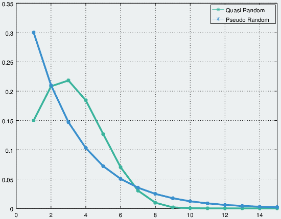
QRNG and PRNG distributions, for p=0.3. The base probability for the QRNG was set to 0.15, and the increment was set to 0.095.
Changing Parameters
Changing the base probability parameter has a fairly obvious affect: it shifts the distribution by the amount the base parameter was changed. At the tail end the changes are marginally more interesting as it can cause the sequence to reach the maximum probability more quickly. The more interesting parameter, however, is the increment as this is what determines the overall shape of the distribution. The graph below demonstrates the effects of varying the increment, but keeping the same base value of 10%:
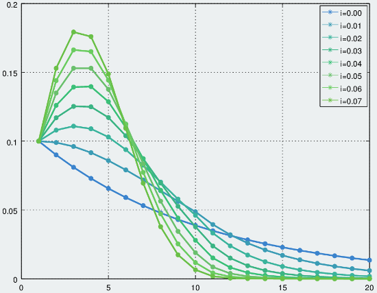
Increments of 0.00 to 0.07 with a base probability of 0.1
A larger increment causes a steeper peak in the distribution, and thus a sharper, faster fall-off towards 0 on the tail end. The case where the increment is 0.0 is effectively a uniform distribution.
Tweaking the maximum probability parameter also affects the shape of the peak, primarily on the downward sloping side. A smaller max value smooths out the tail end of the distribution more. This results in a slightly sharper initial falloff which slows down faster. For example, the following graph shows two curves, both from a quasi-random distribution with base and increment of 0.1. The max state probability is set to 0.46 for the blue curve, and 0.52 for the green curve.
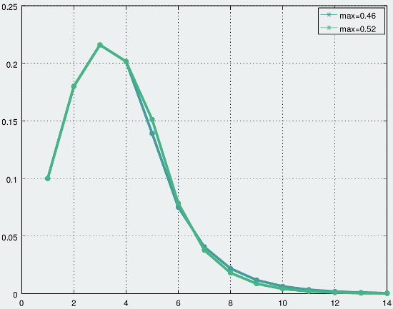
The effect of the max parameter on QRNG distribution shape, with b=0.1 and i=0.1
Extensions
There are a couple of things I need to finish, after which I’ll post my QRNG implementation on GitHub. I’d like to be able to use non-linear increments in the state machine to see what sort of effects they have on the overall distribution. For example a quadratic increment of the form b + ai2. I suspect it won’t really improve anything, but there may be some interesting results.
Additionally, I need to write a tool that can produce distribution parameters that achieve a specific effective probability. Right now I use a sort of trial and error approach to determine the values of b, i and m. My current calibration process involves testing a parameter configuration by sampling the distribution and then tweaking the values accordingly. This process could be automated to some degree, which would desirable when using the QRNG for practical applications.