Table of Contents

Recap

This post took a bit longer to write than originally anticipated, primarily because I was visiting my family for the Christmas holidays. I’m now back at home so work on the series is back on track. To compensate for the delays on publishing Part 3, I’ll try to have Part 4 up in a few days as well.

To recap, the last post in the series discussed several parameters that can be used to tweak the behavior of the convolution operator. This post will build on that knowledge by presenting some of the kernels that show up frequently in image processing. All of the kernels discussed can be tested in the convolution tool.

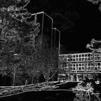
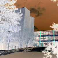
kirsch edge detection, inversion and sharpening filters

Blurring: Box and Gaussian

Blurring parts of an image is a fairly common operation in many contexts, including video games and photo editing. As such, there are numerous different techniques that can be applied to achieve the desired effect. Some blurring methods, such as motion blur and depth of field, require velocity and depth information from a 3D scene to function correctly. Both are often implemented without the explicit use of a kernel. On the other hand, the Gaussian blur and box blur/smooth blur techniques are simple kernel functions that can be applied to any image.

The box blur is by far the simplest of the two techniques; it’s just an nxn matrix filled with ones. After normalization, each matrix element has the value ¹/_n². For example, a 3x3 box blur and its normalized counterpart:

The intuition behind how the blur works is also straightforward — each pixel in the blurred image is the average of the pixel and its neighbors in the source image. Increasing the size of the kernel includes more pixels in the average, so the blur effect is stronger:

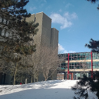
the same image without any filtering, after a 3x3 box blur and after a 9x9 box blur

One advantage of the box blur is that a full kernel matrix isn’t needed. Since every element of the matrix is the same, a shader specifically for applying box blurs can simply use a single uniform int parameter to set the desired blur size.

The Gaussian blur can be seen as a refinement of the basic box blur — in fact, both techniques fall in the category of weighted average blurs. In the case of the box blur each kernel element uses the same weight, however a Gaussian kernel uses weights selected from a normal distribution. A larger weight is assigned to the central element, with elements further from the center having smaller weights. The exact values of the weights depend on the standard deviation chosen for the normal distribution. Usually the distribution mean is set to zero, but a non-zero mean could be used for asymmetric blurring. The rest of this discussion will refer to the function norm(s) which samples a normal distribution with a mean of zero and standard deviation of s.

To produce an nxn Gaussian kernel the distribution is first sampled and stored in an nx1 vector v. Each sample is the integral over the distribution function in the range [-0.5, 0.5] centered around the sample point. The vector is them multiplied with itself to produce the full nxn kernel. Formally:

For example, for a 5x5 Gaussian blur the following discrete distribution is produced:

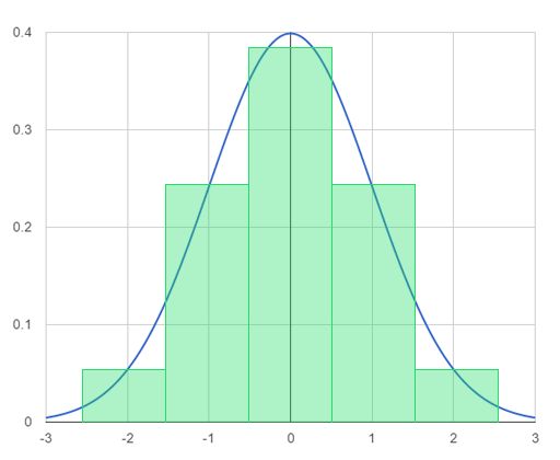
This results in the following vector and kernel matrix:

Like box blurs, increasing the kernel size will make the blur more intense. Increasing the standard deviation will produce a flatter normal distribution, which increases the contribution of pixels on the edge of the convolution. Gaussian blurs produce smoother looking results than box blurs and are more configurable. As such, the technique is one of the most widely used blurring methods in image processing. The fact that the Gaussian kernel is the product of two vectors can be exploited to improve performance. This property will be explored in the next post on separable kernels.

the same image without any filtering, after a 9x9 box blur and after a 9x9 Gaussian blur

The convolution tool has examples of both a 9x9 box blur and a 9x9 Gaussian blur.

Edge Detection: Sobel, Prewitt and Kirsch

One of the techniques that’s be covered extensively in the series is edge detection. So far we’ve only looked at a basic edge detection kernel; the results of the kernel are adequate, but can be improved. Three other common algorithms that produce better results are the Sobel, Prewitt and Kirsch operators. All three of the operators require multiple convolutions — they cannot be implemented using a single kernel invocation.

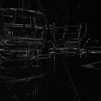
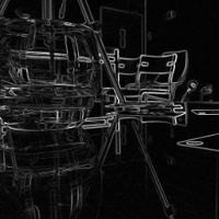
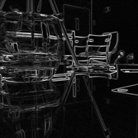
comparison of simple, sobel, prewitt and kirsch edge detection filters

The Sobel and Prewitt techniques are quite similar to each other. Both perform a pair of horizontal and vertical convolutions, which are then used to produce a final edge value at the target pixel. Rather than considering just two axes, the Kirsch edge detector performs a convolution for each of the 8 compass directions at the target pixel. The result with the largest value is retained as the final result for the pixel. The Wikipedia article and convolution tool both cover the details of the kernels involved, so I’ll avoid repeating the information again here.

The convolution tool has examples of all three of the specialized edge detection techniques: Sobel, Prewitt and Kirsch. Custom shaders are used for each of the operators because they’re implemented with multiple convolution passes.

Sharpen: Simple and Unsharp

Sharpening is another common image operation. The technique is used to bring out detail in an image by enhancing the contrast of pixels on edges. Consequently, the simplest method of sharpening an image is to extend the basic edge detector discussed several times in this series. The kernel can be constructed by adding the source image to the edge detector output, producing an image where the edges are more apparent. The sharpening effect can be controlled by introducing an amount parameter that scales the edge detector contribution:

In its most basic form, when amount is set to one, the kernel is as follows:

When amount is zero the sharpening has no effect; larger values result in a strong effect.

comparison of unfiltered image and sharpened images with amount=2 and amount=8

Although easy to construct, a naive sharpen filter tends to have noise and artifacts. The Unsharp Mask technique produces better results and has more options to configure the kernel behavior:

comparison of an unfiltered image, an unsharp filter and a simple sharpen filter

The term “unsharp” comes from the fact that the kernel combines both an edge detector and blur filter, which results in a more refined sharpening effect. Fewer artifacts are produced, so the technique is usually the preferred way to sharpen images. The use of a Gaussian blur is apparent in the following 5x5 unsharp kernel:

Typically an unsharp kernel is configured using three parameters. The first is the amount parameter which is inherited from the simple sharpen kernel. A new radius parameter controls the size of the Gaussian blur and sharpen kernel — a larger radius will result in a larger blur area, causing more pixels to be included. Many implementation also include a threshold value, which is used to specify the minimum difference between two pixels before they’re considered to be an edge.

A more in-depth discussion of where the kernel comes from can be found here. The GIMP manual also has some useful information, though much of it is aimed towards GIMP users.

The convolution tool has examples of both simple and unsharp filters for image sharpening. Only preconfigured kernels are used — there is currently no support for custom amount, radius and threshold values.

Wrap Up

There are plenty of other useful kernels that weren’t discussed in this post. The ImageMagick documentation includes a lengthy discussion of the convolution operator and covers a wide range of kernels. The convolution tool has examples of other image effects such as a bloom and inversion, as well as a custom kernel preset for entering a user-defined 9x9 kernel.

The next two posts in this series will focus on the notion of separable kernels, which can offer significant performance improvements when performing a convolution.