Table of Contents

Introduction

One of my side projects earlier in the month involved developing a tool for running images through different kernels. While working on the project I decided to write a series of blog posts on the use of kernels in image processing. The series will cover a wide range of material, starting from basic kernel operations and working towards more advance techniques. Where applicable posts will also discuss OpenGL implementations. The original tool is a great way to observe the behavior of different kernels; a link to the tool is included in the Table of Contents, and the tool will be referenced directly in other posts.

This post serves as a sort of primer to familiarize the reader with the concepts of a kernel and convolution. Readers already familiar with the topics may not need to read this post at all. All of the posts in the series assume a basic familiarity with matrix and vector algebra. Discussions relating to OpenGL assume that the reader is at least somewhat familiar with the GL shader pipeline and general concepts in computer graphics.

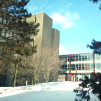
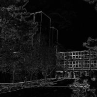
Bloom, blur and edge detection - three operations that can be performed using a kernel

Pixels, Neighbors and Edge Detection

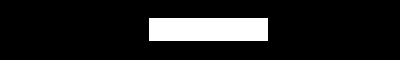
A common procedure in image processing is to apply operations to a pixel based on the value of neighboring pixels. One typical use of this is to identify the edges of objects — not surprisingly, the process is referred to as edge detection. Consider the following one-dimensional subsection of an image:

Even without knowing the full contents of the source image, it’s quite clear that some sort of edge exists where the white and black pixels meet. It might be white text on a dark background or the junction between a wall and a window, but our edge detection procedure should be able to operate without any context. For simplicity, we can assume that the image (and the next few images in this discussion) are composed only of black pixels with a value of 0 and white pixels with a value of 1. Values outside of the range, such as -1 and 2, will be clamped to nearest valid value.

Designing an edge detector for the above image is quite simple. As suggested earlier, the detector should be able to determine if a pixel is an edge based on the value at that pixel and the value of nearby pixels. Ideally we’d like to inspect as few neighboring pixels as possible. In this case only one neighbor is needed — the detector can look for white pixels that have a black pixel immediately to the left. Three different pixel patterns can occur in our single-neighbor system: 00, 01 and 11. The first value in the pattern is the neighbor pixel and the second value is the target pixel. Strictly speaking the pattern 10 is also possible, however it will be omitted for now since it doesn’t occur in the sample image. Only the second pattern, 01, should be identified as an edge. This can be achieved by evaluating the following expression for each pixel, where x is the index of the target pixel and pixels is the array of image data:

In both the 00 and 11 cases the expression evaluates to 0, but in the 01 case it evaluates to 1. One problem is that we haven’t defined a way to handle out of bounds access — if the expression is applied to 0^th pixel in the image, the edge detector will attempt to access the value of the a pixel at an index of -1. We’ll ignore this issue for now as it will be discussed in a later section. There is another larger problem than needs addressing first. In its current state our edge detector can only detect one pattern, which isn’t immensely useful in the general case. It would fail to find both edges in the following image, for example, because one of the edges forms the 10 pattern ignored earlier:

We need to find a way to handle both the 01 and 10 cases with the same detector. This can be done by considering both the left and right neighbors of each pixel — the edge criteria is therefore a white pixel with at least one black neighbor. The number of possible arrangements of pixels increases to 8: 000, 001, 010, 011, 100, 101, 110 and 111. The current pixel is an edge if the pattern is one of 010, 011 and 110; in other patterns, the edge detector should ignore the pixel. To account for the new pattern the edge detector now looks like:

This produces the following results for each of the patterns, after applying the clamping rules:

Thus far the edge detector has only been used on one dimensional images. It wouldn’t work properly on the following image since it has edges spanning both the x and y axis:

There are too many pixel combinations to list, but one case that a 2D detector should consider an edge is the following arrangement:

The same technique used to extend the detector earlier can be applied once again, this time adding the “upper” and “lower” neighbors to the list of pixels considered. As before our detector will look for white pixels with a non-zero number of black neighbors. Since the neighbors are no longer constrained to the horizontal axis, the image needs to be accessed as 2D data using a pair of indices. The four-neighbor edge detector can be written as:

We could conceivably extend the detector further to account for diagonal neighbors, which would result in an expression with nine terms. To reduce complexity and increase readability, a better system for describing neighbor-dependent operations is clearly needed.

Kernels and Convolution

Rather than writing the expression as a sequence of arithmetic operations it can instead be described using a matrix of values. This matrix is referred to as a kernel, mask or convolution matrix. For example, the four-neighbor edge detector derived in the previous section could be written in the following 3x3 form:

Like the old edge detector, a kernel can be applied at a given position in an input image. The kernel is first centered over the target pixel, so that its middle element is aligned with the target. A component-wise multiplication is then performed between the values in the kernel and the image subsection below it. The results of the multiplications are summed to produce a single scalar value. Typically a kernel is evaluated at every pixel in the input and the resulting values are return as a new image.

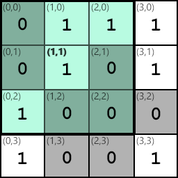
For example assume we have the following 4x4 image:

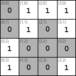
We can apply the edge detector at coordinate (1,1); the blue region highlights the area that will be multiplied with the kernel:

Doing so produces the following computation, ignoring output value clamping:

Similar steps can be taken to apply the kernel at different locations in the image. The results of applying the kernel are collected in another output image:

It’s important to note that although the kernel and image data are stored in matrices, no matrix multiplication is performed. Each value K_i,j in the kernel is multiplied by the corresponding value I_i,j in the image subsection and then added to the running total. Applying a kernel is like a dot product between the kernel and the image.

The process of applying a kernel to an image is referred to as convolution. The name and procedure are somewhat based on the mathematical convolution operation defined for pairs of functions. Formally, for a kernel K of size mxn, input image I and output image O, the convolution between K and I into O can be described as

Out of Bounds Pixels

One of the issues discussed at the beginning of this post was that convolution seems to perform out of bounds accesses on image data. This is indeed the case — when applying a 3x3 kernel at coordinate (0,0), the operation will attempt to access image data at (-1, -1). A simple approach to solving the problem is to only apply the kernel at coordinates with a sufficient number of neighbors in all directions. That is, for an mxn kernel, the first convolution would be performed at the coordinate (floor(m/2), floor(n/2)) rather than (0,0). An example of this can be seen in the animated .gif in the previous section; the edge detector is only applied to coordinates (1,1), (1,2), (2,1) and (2,2).

This works well for some applications, however it results in a decrease in image size. In the 3x3 case a border region of one pixel is ignored, resulting in a loss of 2 pixels of size in both the x and y axes. If multiple convolutions are to applied sequentially, say a set of ten 3x3 kernels, each of these would incur the same loss resulting in 20 pixels of lost resolution in both dimensions.

In many computer graphics applications the resolution loss is problematic. Consider the case of applying a blur effect in a video game, which is typically done as a post-processing step. The original scene might be rendered at a resolution of 1920x1080, after which a Gaussian blur kernel is applied. If the kernel results in a loss of resolution, to 1918x1078 pixels for example, the frame will no longer properly fit to the player’s 1080p screen. To mitigate this the frame could be rendered at a resolution of 1922x1082, but then the frame size becomes tied to size of the post processing kernel. If the kernel changes or multiple kernels of different sizes are used, the solution becomes much harder to manage.

Another way to solve the out of bounds issue that preserves image resolution is to use some method of extending the source image to meet the size requirements of the kernel. In OpenGL (and DirectX) this is quite straightforward to do — out-of-bounds texture access is well defined and can be configured using the relevant texture wrap settings. Two main types of wrapping are available: clamping and repeating. Extending the image with a clamp setting will cause the edge pixels of the image to be returned for all out-of-bounds indices. Repeat wrapping, on the other hand, causes the image to repeat like a tile:

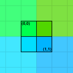
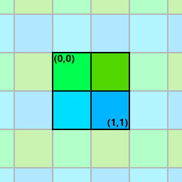
Clamp and repeat texture wrap settings

A third option is to assign all out-of-bounds pixels some preset value such as 0. In OpenGL this should be doable with GL_TEXTURE_BORDER_COLOR settings, although borders aren’t available in WebGL so I haven’t tried it myself. For image effects like blurring this is generally not desirable since it creates a noticeable halo around the edge of the image in the same color as the out-of-bounds pixels. The technique may work fine for other uses such as edge detection however, and I’ve read about it being used for non-image based convolutions in CNNs.

Convolution in OpenGL

The following fragment shader demonstrates one possible implementation of a convolution operator in OpenGL:

uniform float uKernel[9];
uniform sampler2D uSampler;
uniform vec2 uTextureSize;

varying vec2 vTexCoord;

void main(void)
{
    vec4 sum = vec4(0.0);
    vec2 stepSize = 1.0/(uTextureSize);

    sum += texture2D(uSampler, vec2(vTexCoord.x - stepSize.x, vTexCoord.y - stepSize.y))
            * uKernel[0];
    sum += texture2D(uSampler, vec2(vTexCoord.x, vTexCoord.y - stepSize.y))
            * uKernel[1];
    sum += texture2D(uSampler, vec2(vTexCoord.x + stepSize.x, vTexCoord.y - stepSize.y))
            * uKernel[2];

    sum += texture2D(uSampler, vec2(vTexCoord.x - stepSize.x, vTexCoord.y))
            * uKernel[3];
    sum += texture2D(uSampler, vec2(vTexCoord.x, vTexCoord.y))
            * uKernel[4];
    sum += texture2D(uSampler, vec2(vTexCoord.x + stepSize.x, vTexCoord.y))
            * uKernel[5];

    sum += texture2D(uSampler, vec2(vTexCoord.x - stepSize.x, vTexCoord.y + stepSize.y))
            * uKernel[6];
    sum += texture2D(uSampler, vec2(vTexCoord.x, vTexCoord.y + stepSize.y))
            * uKernel[7];
    sum += texture2D(uSampler, vec2(vTexCoord.x + stepSize.x, vTexCoord.y + stepSize.y))
            * uKernel[8];

    sum.a = 1.0;

    gl_FragColor = sum;
}

The shader takes as input a 3x3 kernel, stored in the float array uKernel. uSampler is the source texture sampler that the kernel will be applied to and uTextureSize is the size of the texture. If the shader is written using a GLSL version that supports the textureSize function, the step calculation can be done without the need for a uniform:

ivec2 texSize = textureSize(uSampler, 0);
vec2 stepSize = 1.0 / vec2(float(texSize.x), float(texSize.y));

This makes it possible to get rid of uTextureSize altogether. The texture coordinates stored in vTexCoord indicate which pixel of the texture the fragment shader should process. At each pixel, the fragment shader performs the convolution operation by sampling the source texture 9 times and multiplying by the respective kernel values.

Writing a single fragment shader that can accommodate a wide range of kernel dimensions can be somewhat tricky. One approach is to make all kernels the same size — a 3x3 kernel can be padded with zeros to make it a 9x9 kernel, for example. A fragment shader that can handle 9x9 kernels will work for all kernels of a smaller size as well. However, this means that all convolutions will perform a total of 9x9=81 texture look-ups per pixel, which is less than ideal from a performance standpoint. Branching when kernel values equal zero to avoid texture look-ups is also not great for performance. Another option is to store the kernels in a texture instead of an array. I haven’t tried this so I can’t comment on how well it works, but care would need to be taken to ensure that texture filtering doesn’t affect the kernel values.

To support kernels of different sizes it’s probably easiest to use multiple fragment shaders. For the convolution tool I used the up-scaling approach described because performance wasn’t really important for my application. The convolution is only performed once on the image, until the user changes the settings, so nothing has to run at interactive frame rates. For a real-time application like a game the scaling technique is less feasible.

Wrap-Up

In this post we looked at the motivation behind the use of kernels for image processing and the basics of the convolution operator. All of the kernels introduced in this post were square matrices of size 3x3 — in practice kernels can be any size and have non-square dimensions. In Part 2 of this series some additional properties of kernels will be explored, as well as some useful ways to extend the convolution operation.